MULTI-ANGLE DYNAMIC LIGHT SCATTERING

This application is a national stage application under 35 USC 371 of International Application No. PCT/EP2019/052946, filed Feb. 6, 2019, which claims the priority of European Application No. 18155428.8, filed Feb. 6, 2018, the entire contents of each of which are incorporated herein by reference.

The present invention relates to a method for determining particle size from a multi-angle dynamic light scattering measurement.

Dynamic light scattering is a widely used method for analysing particles in which a time series of measurements of scattered light is used to determine a size or size distribution of particles. Particle characteristics are inferred from the temporal variation in the scattered light. Typically, an autocorrelation is performed on the time series of scattered light intensity, and a fit (e.g. Cumulants, CONTIN, NNLS/non-negative least squares) is performed to the autocorrelation function to determine particle characteristics. Alternatively, a fourier transform may be used to determine a power spectrum of the scattered light, and an analogous fit to the power spectrum performed to determine particle characteristics. Typically, light scattered in a single, well-defined, angle is used in a dynamic light scattering measurement.

Multi-angle dynamic light scattering (MADLS) measurements may also be performed, in which light scattered at more than one angle is used in a dynamic light scattering measurement (Bryant, Gary, and John C. Thomas. “Improved particle size distribution measurements using multiangle dynamic light scattering.” Langmuir 11.7 (1995): 2480-2485).

When multiple scattering angles are used, it is necessary to determine particle characteristics that are most consistent with the scattering data obtained at each scattering angle. There is considerable room for improvement in the existing techniques for doing this.

According to a first aspect, there is provided a method of determining particle size distribution from multi-angle dynamic light scattering data, comprising solving an equation of the form:

[g(θ1)…g(θn)]=[α1K(θ1)…αnK(θn)]x

wherein g(θ_i) is the measured correlation function at angle i, K(θ_i) is the instrument scattering matrix computed for angle i, x is the particle size distribution, and α_iis the scaling coefficient for angle i.

The method comprising using the steps:

a) providing initial estimates for scaling factors α₂to α_n, and defining α₁=1;

b) iterating scaling factors α₂to α_nusing a non-linear solver;

c) solving for x using a linear solver;

d) calculate residual

e) repeat steps b) to d) while the residual is greater than a predefined exit tolerance.

The linear solver may be NNLS, and/or the non-linear solver may be selected from Nelder-Mead simplex, Levenberg-Marquardt and Gauss-Newton.

The initial estimates for the scaling factors α_i(e.g. α₂to α_n) may be estimated by extrapolation of a correlation function g(θi) to a zero-delay time (τ=0).

In some embodiments α₁may not be defined as 1.

The predefined exit tolerance may be: a convergence criterion based on the preceding residual, or an absolute residual threshold.

The method may further comprise repeating the steps a) to e) for a different non-linear solver, to determine which non-linear solver provides the smallest residual.

The method may further comprise measuring a time history of scattered light intensity at each respective scattering angle, θ, and determining the correlation functions g(θ_i) for each scattering angle.

According to a second aspect, there is provided a method of determining particle size distribution from dynamic light scattering data, comprising:

obtaining a measured correlation functions g(θ₁) to g(θ_n); and

solving an equation of the form:

[g(θ1)…g(θn)]=[α1K(θ1)…αnK(θn)]x

wherein:

• • g(θ_i) is the measured correlation function for measurement time i, corresponding with a scattering angle θ_i, K(θ_i) is the instrument scattering matrix computed for the angle θ_i, x is the particle size distribution and α_iis the scaling coefficient for measurement time i (with α₁=1);
  • the vector x takes the form: [x₁, . . . , x_N, n₁, . . . , n_n], where x₁to x_Nare the scattering intensities corresponding with each particle size bin, and the terms n₁to n_nare noise intensities corresponding with each of the measurement times or angles; and
  • columns in K are computed as the expected instrument response according to each element in x, with columns in K at indexes according to elements x₁to x_Ncalculated for each correlator lag-time, τ and angle, θ, and columns at indexes n₁to n_ncalculated as a computed noise contribution at each angle, θ, based on an assumption about the characteristics of the noise.

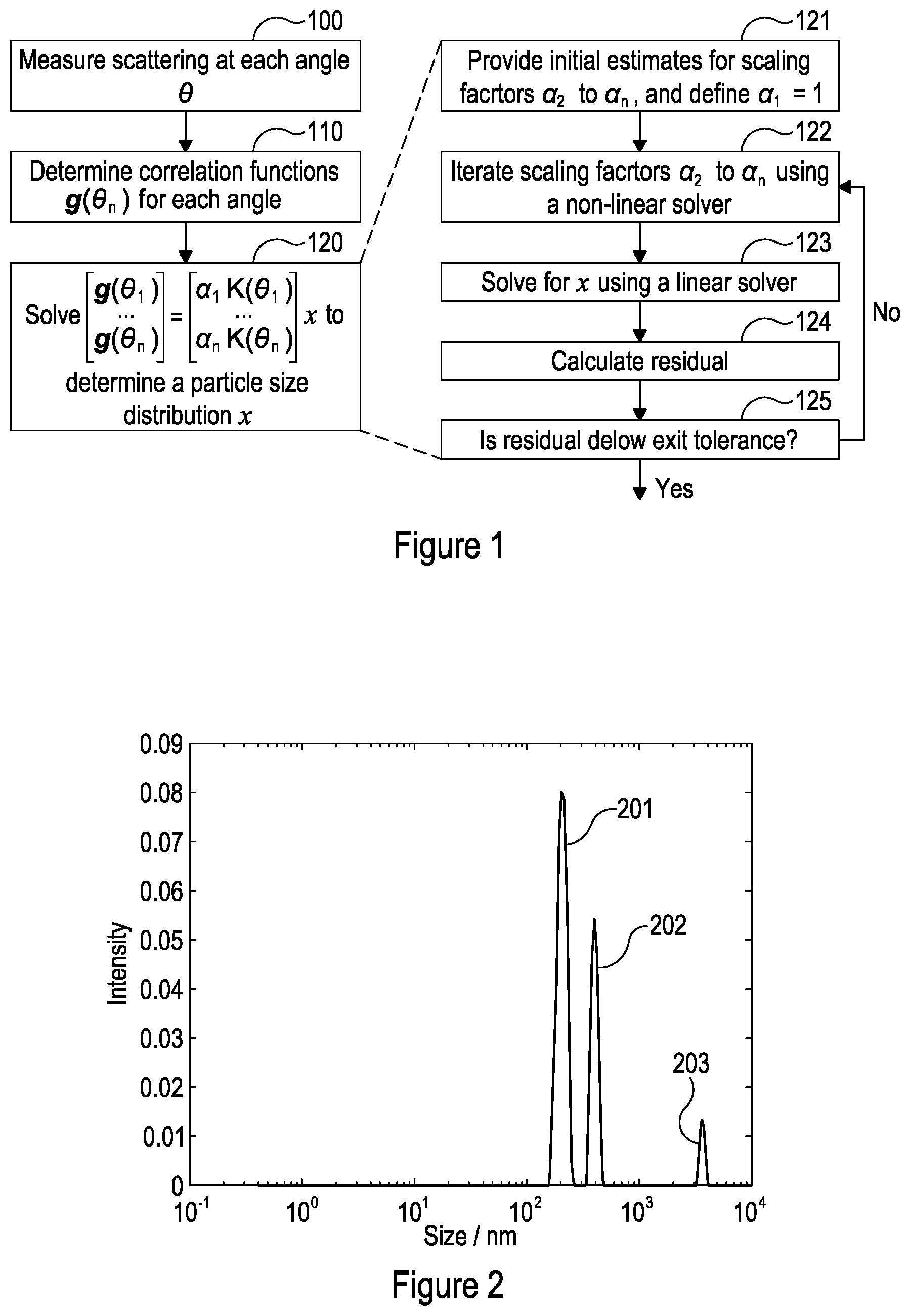
The dynamic light scattering data may be multi-angle data, and each measurement time corresponds with a different measurement angle θ_i; or the dynamic light scattering data may be single angle data, and each measurement time i corresponds with the same measurement angle θ_i. In other embodiments, a combination of same angle and different angle data may be used in the analysis.

The particle size distribution may be determined according to the first aspect, including any of the optional features thereof.

The computed noise contribution may be based on the expected instrument response to a large particle in a scattering volume of the instrument. The large particle may be assumed to be at least 3 microns in diameter, or at least 10 microns in diameter.

The computed noise contribution may be determined according to:

g₁(τ)=exp(−q_i²D_tτ)

where:

g₁(τ) is the instrument-measured field autocorrelation functions at lag time, τ; q is the scattering wave vector

(q=4πn0λsin(θi2));

n₀is the dispersant refractive index; λ is the vacuum wavelength; θ_iis the scattering angle; D_tis the translational diffusion coefficient

(Dt=kBT3πηd);

k_Bis the Boltzmann constant; T is the absolute temperature; η is the dispersant viscosity; and d is the assumed large particle hydrodynamic diameter.

The method may further comprise sequentially measuring a time history of scattered light intensity at each respective time and/or scattering angle, θ, and determining the correlation functions g(θ_n) for each time and/or scattering angle.

According to a third aspect, there is provided a method of determining a particle size distribution, x, from a dynamic light scattering measurement, comprising:

obtaining a correlation function, g, derived from a time sequence of scattering intensity;

solving a system of linear equations comprising:

[g0]=[KγΓ]x

by minimising the sum of residuals:

∥Kx−g∥²+∥γΓx∥²

where K is an instrument scattering matrix, Γ is a regularisation matrix, and γ is a regularisation vector comprising regularisation coefficients for each particle size in the particle size distribution, x.

The method may further comprise performing a measurement to obtain the time sequence of scattering intensity.

The system of linear equations to be solved may include regularisation, thereby comprising:

[g(θ1)…g(θn)0]=[α1K(θ1)…αnK(θn)γΓ]x

wherein the system of equations is solved using steps a) to e), as defined in the first aspect, and in combination with any of the optional features of the first aspect.

Optionally, in the third aspect:

the vector x takes the form: [x₁, . . . , x_N, n₁, . . . , n_n], where x₁to x_Nare the scattering intensities corresponding with each size bin, and the terms n₁to n_nare noise intensities corresponding with each of the measurement times or angles; and

columns in K are computed as the expected instrument response according to each element in x, with columns in K at indexes according to elements x₁to x_Ncalculated for each correlator lag-time, τ and angle, θ, and columns at indexes n₁to n_ncalculated as a computed noise contribution, at each angle, θ, based on an assumption about the characteristics of the noise.

According to a fourth aspect, there is provided a machine readable medium, comprising instructions for causing a processor to perform the method of any of the preceding aspects.

According to a fifth aspect, there is provided an instrument for performing a DLS measurement, comprising: a light source, a sample holder, a detector, and a processor; wherein:

the light source is configured to illuminate a sample in the sample holder with a light beam to produce scattered light from the interaction of the light beam with particles suspended in the sample holder by a fluid;

the detector is configured to detect the scattered light and to provide measurement data to the processor,

the processor is configured to process the measurement data to determine a particle size distribution using a method according to any of the first, second or third aspects, including any optional features thereof.

Each of the features of each aspect (including optional features) may be combined with those of any other aspect.

When performing a MADLS measurement with three measurement angles (θ₁, θ₂and θ₃) the following system of linear equations must be solved (with only the relevant matrix components shown):

[g(θ1)g(θ2)g(θ3)]=[K(θ1)aK(θ2)bK(θ1)]x(1)

Where g(θ_i) is the measured correlation function at angle i, K(θ_i) is the instrument scattering matrix computed for angle i, and x is the particle size distribution. The aim is to determine the particle size distribution from the measured correlation functions. The coefficients a and b are scaling factors, and initial estimates for these can be calculated by extrapolation (linear or otherwise) of the correlation function to time-zero to determine the y-axis multiplier. The physical origin of a and b is the sum of the scattered intensity into each angle.

Note that the first scattering angle θ₁has arbitrarily been chosen as the measurement angle to which the other measurement angles are scaled. It will be appreciated that any of the other measurement angles could alternatively be selected as having a unitary scaling factor, and the other measurement angles scaled to that angle.

Bryant (referenced above) discloses deriving a and b from the count rate, and the use of a linear solver, but this method is prone to error if the count rate is not stationary over time. Cummins (P. G. Cummins, E. J. Staples, Particle Size Distributions Determined by a “Multiangle” Analysis of Photon Correlation Spectroscopy Data, Langmuir, 1987, 3, 1109-1113) discloses using a non-linear solver to determine a, b and x. Applying a non-linear solver in this way is problematic, because there are a large number of coefficients (in x) to be determined and there is a significant possibility that the solution will not converge reliably.

In embodiments of the present invention, a nested approach is used, in which a non-linear solver (such as Nelder-Mead simplex, Levenberg-Marquardt, Gauss-Newton or another method) is used to iterate an estimate for a and b, and within each non-linear iteration, a linear solver (e.g. non-negative least squares) is used to determine a best fit for x and consequently determine a residual error. The residual error is then used by the non-linear solver to select new values for each of the scaling factors. This is exemplified in the following pseudo-code:

This nested technique allows a fast and robust linear method (e.g. NNLS) to be applied to the linear problem of solving the particle distribution. Coefficients a and b are variable scalars that require a non-linear approach, and a non-linear solver is therefore appropriate for this. This approach is preferable over tackling the entire problem with a non-linear solver (the approach taken by Cummins). Embodiments therefore provide more robust, faster to execute, solutions for MADLS. This in turn enables a larger number of size classes (i.e. a longer vector x), so that MADLS can be used to span a greater size range than in the literature, or to provide a particle size distribution with a greater resolution than in the prior art.

This method can be generalised to apply to the following set of equations, for n number of scattering angles:

[g(θ1)…g(θn)]=[α1K(θ1)…αnK(θn)]x(2)

With α_icorresponding with the scaling coefficient for angle i.

Conventionally, the first scattering (i=1) angle may have a scaling coefficient defined as 1 (α₁=1). As mentioned above, this is merely an arbitrary convention: in alternative embodiments the scaling may be performed relative to any of the measurements 1 to n. It will also be appreciated that the order of concatenation of measurement results is also arbitrary, and any of the measurements may be placed first. For ease of notation, the scaling mentioned herein is denoted as relative to the first measurement, but this does not imply a limitation.

The generalised pseudo code therefore becomes:

In each iteration of the non-linear solver (e.g. Levenberg-Marquart, etc.), the estimate for each of the scaling coefficients α₂to α_nis updated before a new estimate for the particle size distribution x is determined using a linear solver such as NNLS, and the new estimate of particle size distribution is used to calculate a residual. The residual is both used by the non-linear solver in the next iteration to select the new estimates for the scaling factors, and to determine if the estimates are acceptable. This work flow means that the problem is efficiently partitioned so that the scaling factors can be accurately and efficiently determined.

FIG. 1 schematically illustrates a method of determining a particle size distribution according to an embodiment. At step 100, a time series of scattering intensity is measured (or determined from a time history of photon arrival times) at each scattering angle (e.g. sequentially, or in some embodiments, simultaneously). At step 110, correlation functions are determined for each scattering angle from the respective time series of scattering intensity (e.g. using a correlator). At step 120, the equation (2) is solved to determine a particle size distribution x.

The process of solving equation (2) to determine the particle size distribution comprises:

at step 121, determining initial estimates for scaling factors α₂to α_n, and defining α₁=1;

at step 122, iterating scaling factors α₂to α_nusing a non-linear solver;

at step 123, solving for x using a linear solver;

at step 124, calculate residual

at step 125, check whether the residual is greater than a predefined exit tolerance.

When performing a multi-angle DLS measurement, the data that is measured at each angle must be representative of the same sample. In most measurements, it can be assumed that the sample will not change over the duration of the measurement. If Typically, because of the relatively high cost of suitable detectors for DLS (which typically employs a photon counting detector such as an avalanche photodiode) the scattering measurements at each angle are taken sequentially, with an optical path to a single detector cycled between each detection angle. Additionally, due to the field of view of the detector, different measurement angles sample a subtly different scattering volume, even if the volume centres are coincident. Under these measurement circumstances, a transient contaminant (such as dust, or filter debris) will tend to contaminate a single scattering angle. This will adversely affect the result, since it will not be possible to find a common solution that satisfies the measurement data (because one of the measurements is not representative of the sample).

It is possible to accommodate the presence of noise at a single angle during the fitting process by including terms (specific to the noise type) in the solution that depend each only on a single angle. The particle size distribution result should remain common across all angles. Noise usually manifests as a slowly decaying contribution to the correlogram caused by dust at one measurement angle. However, noise types of any form can be accounted for if they are suspected to exist.

As already discussed above, the regular system of linear equations is of the form g=Kx, where g is the measured correlation function, K is the instrument scattering matrix, and x is the particle size distribution (neglecting the scaling factor coefficients for simplicity of notation).

With application to MADLS, the equation becomes (with only the relevant matrix components shown):

[g(θ1)…g(θn)]=[K(θ1)…K(θn)]x(3)

In prior art analyses, the vector x comprises a set of N scalar values, each scalar value defining an intensity of scattering from a particular range of particle sizes (or bin). In embodiments of the present invention, the vector x includes at least one additional value that is included to accommodate the presence of contaminants at one or more scattering angle. For n=3, corresponding with three measurement angles, and a particle size distribution comprising N size bins, the vector x may take the following form: [x₁, x₂, x₃, . . . , x_N, n₁, n₂, n₃], where x₁to x_Nare the scattering intensities corresponding with each size bin, and the terms n₁to n₃are noise intensities corresponding with each of the three scattering angles.

The matrix

[K(θ1)…K(θn)]

has the following form: columns in K are computed as the expected instrument response according to each element in x. Columns at indexes according to elements x₁to x_Nmay be calculated theoretically for each correlator lag-time, τ, and angle, θ. Columns at indexes n₁to n₃take the form of a computed noise contribution, at each angle, based on an assumption about the characteristics of the noise.

In an example embodiment, the noise contribution is assumed to take the form of large transient particles in the scattering volume. For example, the model used to estimate the noise contribution columns of K may mimic that used to compute the expected instrument response for a size bin, but use a fixed particle diameter of 10 microns at the particular scattering angle i, and for each correlator lag-time, τ:

g₁(τ)=exp(−q_i²D_tτ)  (4)

Where:

g₁(τ) is the instrument-measured field autocorrelation functions at lag time, τ;

q is the scattering wave vector

(q=4πn0λsin(θi2));

n₀is the dispersant refractive index;

λ is the vacuum wavelength;

θ_iis the scattering angle;

D_tis the translational diffusion coefficient

(Dt=kBT3πηd);

k_Bis the Boltzmann constant;

T is the absolute temperature;

η is the dispersant viscosity; and

d is the particle hydrodynamic diameter.

Since the noise at each angle is not related to the noise at any other measurement angle (for a sequential multi-angle measurement), elements are zero at angles other than for which the noise is considered. If large material is present at just one angle, the solution residual will minimise if intensity is assigned to the noise bin during fitting. The solver will not compromise the particle size distribution fit result by addition of spurious particles.

In an example, a mixture of polystyrene latex spheres of diameter 200 nm and 400 nm was prepared in an aqueous dispersion. Two methods were used to fit a particle size distribution to the same instrument data. The first method did not assume any single-angle noise. FIG. 2 shows the resulting particle size distribution, which comprises a peak 201 at 200 nm, a peak 202 at 400 nm and a peak 203, corresponding with a contaminant, at 3.5 microns. The fit residual has a magnitude of 4.6e-4 (L2-norm).

FIG. 3 shows the vector x calculated in accordance with an embodiment, in which a single-angle noise contribution is assumed to be present to a greater or lesser degree at each scattering angle. The result is a particle size distribution that includes a peak 301 at bins corresponding with 200 nm, a peak 302 at bins corresponding with 400 nm, negligible contaminant at 3.5 microns and significant single-noise contribution 303 in the noise bins that are at the end of the vector x. In this case the noise contribution was present in back-scatter but not in either of side-scatter or forward scatter, as illustrated in FIG. 4, which shows the intensity assigned to contaminants at each of the three scattering angles of this measurement. The fit residual has a magnitude of 3.8e-4 (L²-norm)—smaller than achieved without consideration of a single-angle noise contribution.

Although the foregoing example has illustrated the application of this technique to three scattering angles, it will be understood that fewer or more scattering angles may be used in accordance with alternative embodiments.

In some embodiments, the same principles can be applied to measurements that are not taken at different scattering angles (but are taken at different times, with at least some, or all, at the same scattering angle), so that a particle size distribution can be determined from the ensemble data that discounts scattering contributions from contaminants. This approach will be effective in removing scattering contributions from contaminants that are not present in every measurement, and which are well approximated by the model used to simulate the scattering contribution from the contaminants.

Because the MADLS problem (and more generally, the DLS problem) is ill-conditioned, regularisation may be used to bias the solution against fitting to noise and to enforce some predefined property of the result. The system of linear equations g=Kx becomes (with only the relevant matrix components shown):

[g0]=[KγΓ]x(5)

In the above, g may represent a matrix of n correlation functions

(i.e.[g(θ1)…g(θn)]),

each corresponding with a measurement taken at a different time and/or at a different scattering angle, and K may represent a matrix

[K(θ1)…K(θn)].

Typically, the regularisation coefficient, γ, takes the form of a scalar value to enforce more or less regularisation, dependant on the magnitude of γ, with larger γ resulting in more regularisation. The regularisation matrix, Γ, can take several forms. When performing DLS, it is often desired to enforce smoothness in the result as particle size distributions are believed to be mostly continuous. Alternatively, the solution norm may be biased toward zero if the particle size distribution is believed to be monomodal.

The regularisation term, γΓ, forms part of the residual to be minimised:

∥Kx−g∥²+∥γΓx∥²  (6)

In this example embodiment, the matrix Γ may act as a low pass operator to penalise curvature in the solution, x. When measuring the particle size distribution across a large dynamic range of size bins, it is not always possible to realise a regularisation coefficient that suitably penalises curvature at small particle size and large particle size simultaneously. This is not only in part due to the relative separation of neighbouring size bins (since these are typically log-spaced) but also the differing particle characteristics at small and large particle size.

According to embodiments, this problem may be solved by using a vector of regularisation coefficients γ, such that the regularisation coefficient is dependent on the particle size.

[g0]=[KγΓ]x(7)

This allows more regularisation to be enforced at large sizes where particle size classes are more widely spaced and we wish to prevent a spiky solution. Conversely, this allows less regularisation at small size where we wish to employ more resolving capability. In this way, the highest possible resolution may be maintained across a large size range—0.3 nm to 10 um.

In order to illustrate this, an example DLS measurement will be simulated. The simulated example comprises four separate particle components:

This represents a two-component mixture of protein monomers in the presence of a small number of large particulates (the large particulates are similar by scattering intensity, because this scales with the sixth power of particle diameter). A white noise contribution of 0.1% was added to the simulated auto-correlation functions. Shown in FIG. 5 is the resultant particle size distribution, derived using the MADLS method with a vector of regularisation coefficients. All peaks are resolvable, with peaks 401 to 404 respectively corresponding with peak ID 1 to 4 in the above table.

The vector of regularisation coefficients, γ, employed in the above analysis varied with particle size in a way that is linear in log space, according to the function:

γ_x=m·log(x)+c  (8)

In this example, m=0.019 and c=0.0026 (with x measured in nm), with the result that the regularisation coefficient varied as shown in FIG. 6. Other functions of particle sized may be used to determine the regularisation vector (e.g. a non-log function, a polynomial etc).

The results in FIG. 5 can be contrasted with results obtained with a scalar regularisation coefficient (γ=0.002), which are shown in FIG. 7. In FIG. 7 the large particle contribution is over-resolved because of noise on the simulated measurement.

Increasing the scalar regularisation coefficient (γ=0.0065), does not remedy this problem, because this causes the small particle contribution to be poorly resolved, as shown in FIG. 8. The applicant has found that using a vector regularisation that varies with particle size to provide improved measurement accuracy in the particle size distribution.

It is possible to determine an appropriate regularisation coefficient (e.g. automatically). One method described in the literature is the L-curve method (C. Hansen, D. P. O'Leary, The use of the L-Curve in the Regularization of Discrete Ill-Posed Problems, SIAM J. Sci. Comput., 1993, 14(6), 1487-1503). According to this method, the optimal regularisation coefficient is that which minimises both the residual norm (∥Kx−g∥) and the regularisation norm (∥Γx∥). Plotting the residual norm against the regularisation norm across a range of regularisation coefficient typically results in an L-shaped curve, the corner of which represents the optimum regularisation coefficient.

This approach can be adapted to determine an optimum regularisation vector, γ. In the example above, in which a linear log function is used to determine the regularisation vector, the intercept, c, and the gradient m, can be iterated, and multiple residual norm vs regularisation norm (L-curves) can be plotted. Following this, an appropriate regularisation intercept and gradient pair can be deduced. In principle, a similar analysis can be applied to compare any functions for determining an appropriate regularisation vector. Such an analysis can be applied automatically by a processor/instrument, based on measurement data (simulated or actual) that is representative of a particular use-case for an instrument. Alternatively, a regularisation vector (or vectors) can be determined that is generally appropriate for a particular customer requirement. In some embodiments, the user may be able to select between alternative regularisation approaches (e.g. scalar, first vector (low gradient), second vector (high gradient), etc).

FIG. 9 shows a set of L-curves 501-507 respectively corresponding with values of gradient, m, in equation (8) of 0.003 to 0.009 (in increments of 0.001), with each curve 501-507 having a series of values for intercept, c, incremented between 0.001 and 0.01. Low gradient with moderate intercept are shown by FIG. 9 to be optimal (e.g. similar to the parameters used for FIG. 5).

FIG. 10 illustrates an instrument according to an example embodiment, comprising a light source 10, sample holder 20, detector 30, processor 40 and optional display 50.

The light source 10 may be a laser (or an LED) and illuminates a sample on or in the sample holder 20 with a light beam. The sample comprises a fluid in which particles are suspended, and the light beam is scattered by the particles to create scattered light. The scattered light is detected by the detector 30, which may comprise a photon counting detector such as an APD. Suitable collection optics may be provided to collect light scattered at a particular scattering angle (such as a non-invasive backscatter, or NIBS, arrangement that is employed in the Zetasizer Nano from Malvern Panalytical Ltd). The collection optics may be configured to allow a single detector to receive light scattered at different angles (e.g. using optical fibres and an optical switch).

The detector 30 provides measurement data (e.g. a sequence of photon arrival times) to the processor 40, which may be configured to determine a scattering intensity over time. The processor determines a correlation function from the measurement data, for use in determining particle size in accordance with dynamic light scattering principles. Specifically, the processor 40 is configured to perform at least one of the methods described herein.

The processor 40 is optionally configured to output a particle size distribution to a display 50, which displays the result to a user. The processor 40 may comprise a system on chip/module, a general purpose personal computer, or a server. The processor 40 may be co-located with the detector 30, but this may not always be the case. In some embodiments the processor 40 may be part of a server, to which measurement results are communicated (e.g. by a further computing device).

Although a number of examples have been described, these are not intended to limit the scope of the invention, which is to be determined with reference to the accompanying claims.